Convex Optimization Note(3): Convex Optimization
1. Optimization Formulation
Eliminating Linear Equality Constraints
For a linear equation constraints \(Ax=b\), supposing the corresponding feasible set is \(S=\{x|Ax=b\}\). The constraint can be eliminated by substituting \(x\) with \(x_0+Fz\) where \(x_0\) is a particular solution of \(Ax=b\) and \(F\) is a basis of the null space of \(A\). Thus, we do not need constraints on variable \(z\).
Conditions: \(RF=ker\ A\), \(x_0\in S\)
\[x\in S \iff x-x_0\in ker\ A \iff x-x_0\in RF\iff x-x_0=Fz\]
Null space of matrix \(A\): \(ker\ A=\{x|Ax=0\}\)
Range of matrix \(F\): \(RF=\{Fx|x\in\mathbb{R}^n\}\)
2. Convex Optimization
Basic formulation of convex optimization problem:
\[ \begin{aligned} \min_{x\in\mathbb{R}^n}&f_0(x) \\s.t. &f_i(x)\leq0,\ i=1,...,m \\&a_i^Tx=b_i,\ i=1,...,p \end{aligned} \]
where:
\(f_0, f_1\dots f_m:\mathbb{R}^n\rightarrow\mathbb{R}\) is convex
\(h_i\) is affine
Optimality Conditions
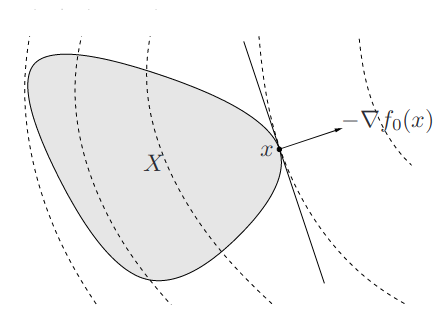
In convex optimization, a local minimum is also a global minimum. The optimal condition is: \[\nabla^Tf(x)(y-x)\geq0,\ \forall y \in\text{feasible set}\] Geometrically, it means that \(-\nabla^Tf(x)\) is a supporting hyperplane of the feabile set at \(x\). (if \(\nabla f(x) \neq 0\))

Unconstrained problem: \(\nabla f(x)=0\)
Problem with only equality constraints: \[ \begin{aligned} \min_{x}\quad&f(x) \\s.t. \quad &Ax=b \end{aligned} \] \(y-x\in \mathcal{N}(A)\) since they are both in the feasible set. Thus, \(\nabla f(x) \perp \mathcal{N}(A)\) > If a linear function is non-negative on a subspace, then it must be zero on this subspace.
Non-negative orthant \[ \begin{aligned} \min_{x}\quad&f(x) \\s.t. \quad &x\succeq 0 \end{aligned} \] After deduction, we can get \(x_i(\nabla f(x))_i= 0\), which is a complementarity condition. This can also be achieved by KKT condition.
Quasi-convex Optimization
Only the cost function is quasi-convex compared to convex optimization. For quasi-convex constraints, we can always find a convex constraints that is equivalent to the original one(same 0-level subset).
\[\nabla^Tf(x)(y-x)>0\quad \forall y\in \mathcal{X}/x \implies x \text{ is global optimal}\]
Only sufficient
gradient non-zero
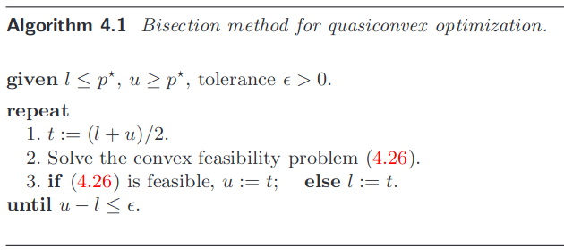
Bisection Method: From quasi-convex to convex optimization
For a quasi-convex problem, we can use bisection method to find the
optimal solution. The idea is to use a convex function family \(\phi_t(x)\) to approximate the original
function \(f(x)\): \[f(x)\leq t \iff \phi_t(x)\leq 0\] Then try
to approximate the optimal solution \(p^*\): 
Linear Optimization
All the constraints and objective are affine.
\[ \begin{aligned} \min\quad & c^Tx+d\\ s.t.\quad & Gx\leq h\\ & Ax=b \end{aligned} \]
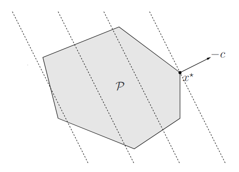
Geometric interpretation of linear optimization: 
Linear-fractional Programming
The objective is a ratio of affine functions: \[ f_0(x)=\frac{c^Tx+d}{e^Tx+f} \] This is a quasi-convex optimization.
Quadratic Optimization
The objective is a quadratic function and the constraints are affine. \[ \begin{aligned} \min\quad & \frac{1}{2}x^TPx+q^Tx+r\\ s.t.\quad & Gx\leq h\\ & Ax=b \end{aligned} \]
If the inequality constraints are quadratic(convex), the problem is
called quadratically constrained quadratic
programming(QCQP). If the constraint can be written as \(||Ax+b||_2\leq c^Tx+d\), it is called
second-order cone programming(SOCP). Their relationship
can be expressed as following: 
Example of a robust linear programming problem: \[ \begin{aligned} \min\quad & c^Tx\\ s.t.\quad & a_i^Tx\leq b_i,\ i=1,...,m \end{aligned} \] The \(a_i\) lie in a elipsoid: \[ \begin{aligned} a_i\in\mathcal{E}_i=\{a_c+P_iu\quad|\quad ||u||_2\leq 1\} \end{aligned} \] The constraint can be reduced to: \[ \begin{aligned} a_c^Tx+||P_i^Tx||_2\leq b_i \end{aligned} \] Which is a SOCP. With similar method, we can transfer a random linear constrained problem into an SOCP problem: \[\textbf{Prob}(a_i^Tx\leq b_i)\geq \Phi\]
Geometric Programming
Forms that are not convex originally but can be transferred into a convex function by its Monomials and Posynomials formed constraints.
Monomials: \(f(x)=cx_1^{a_1}x_2^{a_2}\dots x_i^{a_i}\)
Posynomials: Linear combinations of monomials
Convex Optimization in the form of Generalized Inequality
The standard form of convex optimization can also be expressed through generalized inequality. In the following chapters, we will see this can also be solved as easily as ordinary convex optimization problems. \[ \begin{array}{ll} \operatorname{minimize} & f_0(x) \\ \text { subject to } & f_i(x) \preceq_{ \text { K }_i} 0, \quad i=1, \ldots, m \\ & A x=b, \end{array} \]
Conic Form Problems
The conic form problem is a special case of the generalized inequality problem. It has a linear objective and one affine inequality constraint: \[ \begin{array}{ll} \operatorname{minimize} & c^Tx \\ \text { subject to } & Ax+b \preceq_{ \text { K }} 0 \end{array} \] If \(K\) is the non-negative orthant, the problem is a linear programming problem.
Semi-definite Programming
The semi-definite programming is a special case of the conic form problem when \(K \in S_+^k\) is the cone of positive semi-definite matrices. \[ \begin{array}{ll} \operatorname{minimize} & c^T x \\ \text { subject to } & x_1 F_1+\cdots+x_n F_n+G \preceq 0 \\ & A x=b, \end{array} \]
The inequality constraint is a linear matrix inequality(LMI) if \(F_i,G\) are diagonal.
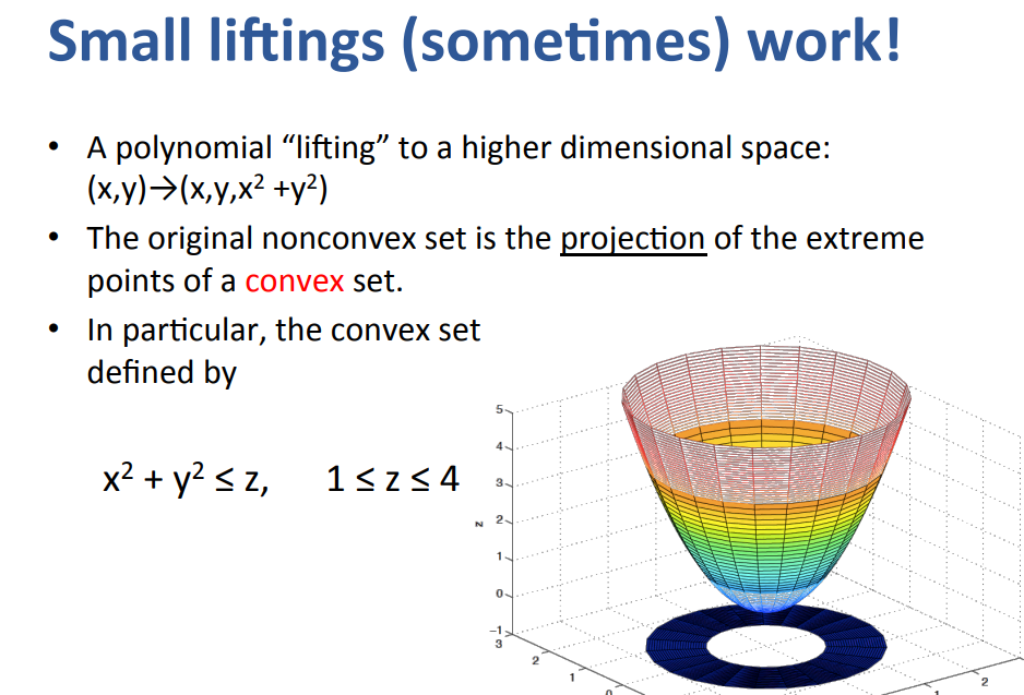
Here is an example of converting a non-convex problem into a semi-definite programming(thus convex) problem through "lifting". It is just a simple example to leave some impression of SDP. We will see more examples in the following chapters. The figure comes from here.
